更高效的支持向量机算法实现及其在手写数字识别中的应用——03不同Kernel的SVM超参数优化

大数据机器学习课程第二次实验项目

本文是更高效的支持向量机算法实现及其在手写数字识别中的应用系列文章第03篇——不同Kernel的SVM超参数优化。

dataset_dict_uci_digits = load_digits(as_frame=False)
X_train, X_val, X_test, y_train, y_val, y_test, train_set, val_set, test_set, data_module, categories = process_sklearn_dataset_dict(dataset_dict_uci_digits, 'all')
# dataset_dict_full_mnist = fetch_openml("mnist_784", as_frame=True)
# X_train_full, X_val_full, X_test_full, y_train_full, y_val_full, y_test_full, train_set_full, val_set_full, test_set_full, data_module_full, categories_full = process_sklearn_dataset_dict(dataset_dict_full_mnist, 'all')

(1797, 64) float32 (1797,) int64 [0 1 2 3 4 5 6 7 8 9]
1293 144 360

0.1 附加题: 对比不同 kernel 方法下的 SVM 分类器 （对完整SVM进行调参）

这一题本质上是让我们以 kernel 的选择（也包括选择线性Kernel）作为目标元参数，其他参数作为冗余或固定元参数，进行调参实验，发现不同 kernel 方法下的 SVM 分类器的分类效果数值上的区别及其显著性，并且从可视化分析上也作出进一步解释。

为了让问题简单清晰，我们再这一节不用我们自己实现的SVM（我们刚才实现的Linear Soft Margin SGD SVM），而是直接使用成熟的经过检验的，刚才我们测试出来最快的 Thunder SVM 库（与sklearn接口兼容，速度更快，使用GPU）。这样我们就可以专注于调参优化问题本身，而不是关注具体实现细节。

0.1.1 科学调参的原则与方法

我在上次Project作业KD树中详细描述了谷歌AI团队《深度学习调优指南》的思想，涉及到的概念包括目标元参数、冗余元参数和固定元参数，贝叶斯优化、演化计算、近似随机搜索，科学实验的控制变量法与调参实验设计中的探索与利用、调参结果的假设检验分析等。这里我们不再赘述，需要的话可以阅读上次作业的文档。

0.1.2 搜索空间定义

我们使用dataclass，要求传入函数的参数是强类型，而且有一个随机概率分布，这样方便定义调参。这里用到我自己写的scholarly_infrastructure库的一个核心功能，对Python标准的dataclass进行了改进。

---

source

SupportVectorClassifierConfig

 SupportVectorClassifierConfig (C:float=1.0, kernel:str='rbf',
                                degree:int=3,
                                gamma:Union[str,float]='scale',
                                coef0:float=0.0, shrinking:bool=True,
                                probability:bool=False, tol:float=0.001,
                                cache_size:float=200, class_weight:Union[d
                                ict,str,NoneType]=None,
                                verbose:bool=False, max_iter:int=-1,
                                decision_function_shape:str='ovr',
                                break_ties:bool=False,
                                random_state:Optional[int]=None)

from scholarly_infrastructure.rv_args.nucleus import RandomVariable, experiment_setting
from optuna.distributions import IntDistribution, FloatDistribution, CategoricalDistribution
from typing import Optional, Union

@experiment_setting
class SupportVectorClassifierConfig:
    # 惩罚系数 C
    C: float = ~RandomVariable(
        default=1.0,
        description="Regularization parameter. The strength of the regularization is inversely proportional to C.",
        distribution=FloatDistribution(1e-5, 1e2, log=True)
    )
    
    # 核函数类型
    kernel: str = ~RandomVariable(
        default="rbf",
        description="Kernel type to be used in the algorithm.",
        distribution=CategoricalDistribution(choices=["linear", "poly", "rbf", "sigmoid",
                                                      "precomputed"
                                                      ])
    )
    
    # 多项式核函数的度数
    degree: int = ~RandomVariable(
        default=3,
        description="Degree of the polynomial kernel function ('poly').",
        distribution=IntDistribution(1, 10, log=False)
    )
    
    # 核函数系数 gamma
    gamma: Union[str, float] = ~RandomVariable(
        default="scale",
        description="Kernel coefficient for 'rbf', 'poly' and 'sigmoid'.",
        distribution=CategoricalDistribution(choices=["scale", "auto"])  # 可以添加浮点数分布视需求
    )
    
    # 核函数独立项 coef0
    coef0: float = ~RandomVariable(
        default=0.0,
        description="Independent term in kernel function. It is significant in 'poly' and 'sigmoid'.",
        distribution=FloatDistribution(0, 1)
    )
    
    # 收缩启发式算法
    shrinking: bool = ~RandomVariable(
        default=True,
        description="Whether to use the shrinking heuristic.",
        distribution=CategoricalDistribution(choices=[True, False])
    )
    
    # 是否启用概率估计
    probability: bool = ~RandomVariable(
        default=False,
        description="Whether to enable probability estimates. Slows down fit when enabled.",
        distribution=CategoricalDistribution(choices=[True, False])
    )
    
    # 停止准则的容差 tol
    tol: float = ~RandomVariable(
        default=1e-3,
        description="Tolerance for stopping criterion.",
        distribution=FloatDistribution(1e-6, 1e-1, log=True)
    )
    
    # 内核缓存的大小（MB）
    cache_size: float = ~RandomVariable(
        default=200,
        description="Specify the size of the kernel cache (in MB).",
        distribution=FloatDistribution(50, 500, log=False)
    )
    
    # 类别权重 class_weight
    class_weight: Optional[Union[dict, str]] = ~RandomVariable(
        default=None,
        description="Set C of class i to class_weight[i]*C or use 'balanced' to adjust weights inversely to class frequencies.",
        distribution=CategoricalDistribution(choices=[None, "balanced"])
    )
    
    # 是否启用详细输出
    verbose: bool = ~RandomVariable(
        default=False,
        description="Enable verbose output (may not work properly in a multithreaded context).",
        distribution=CategoricalDistribution(choices=[True, False])
    )
    
    # 最大迭代次数
    max_iter: int = ~RandomVariable(
        default=-1,
        description="Hard limit on iterations within solver, or -1 for no limit.",
        distribution=IntDistribution(-1, 1000, log=False)
    )
    
    # 决策函数形状
    decision_function_shape: str = ~RandomVariable(
        default="ovr",
        description="Whether to return a one-vs-rest ('ovr') decision function or original one-vs-one ('ovo').",
        distribution=CategoricalDistribution(choices=["ovo", "ovr"])
    )
    
    # 是否打破决策函数平局
    break_ties: bool = ~RandomVariable(
        default=False,
        description="If True, break ties according to the confidence values of decision_function when decision_function_shape='ovr'.",
        distribution=CategoricalDistribution(choices=[True, False])
    )
    
    # 随机种子 random_state
    random_state: Optional[int] = ~RandomVariable(
        default=None,
        description="Controls random number generation for probability estimates. Ignored when probability=False.",
        distribution=IntDistribution(0, 100)  # 根据需求设置范围
    )

# show_dataframe_doc(SupportVectorClassifierConfig)[:1]
SupportVectorClassifierConfig.show_dataframe_doc()[:1]
# SupportVectorClassifierConfig.get_optuna_search_space(frozen_rvs={"verbose", "cache_size", "random_state"})

	name	type	default	default_factory	init	repr	hash	compare	metadata	kw_only	description	distribution
0	C	<class 'float'>	1.0	<dataclasses._MISSING_TYPE object at 0x7f36bc2...	True	True	None	True	None	<dataclasses._MISSING_TYPE object at 0x7f36bc2...	Regularization parameter. The strength of the ...	FloatDistribution(high=100.0, log=True, low=1e...

from dataclasses import asdict

0.1.3 定义目标函数

---

source

evaluate_svm

 evaluate_svm (config:__main__.SupportVectorClassifierConfig, X_train,
               y_train, trial:optuna.trial._trial.Trial=None,
               critical_metric='acc1_pred', num_of_repeated=5)

import optuna
from sklearn.svm import SVC
from sklearn.model_selection import KFold

def evaluate_svm(config:SupportVectorClassifierConfig, X_train, y_train,
                 trial:optuna.Trial = None, 
                 critical_metric="acc1_pred", num_of_repeated=5):
    # 使用k fold交叉验证，相当于做了5次独立实验。
    kf = KFold(n_splits=num_of_repeated, shuffle=True, random_state=config.random_state)
    
    
    result_dict = dict()

    metric_names = set()
    
    # 进行5折交叉验证
    for experiment_index, (train_index, test_index) in enumerate(kf.split(X_train)):
        # 分割训练集和测试集
        X_train_fold, X_test_fold = X_train[train_index], X_train[test_index]
        y_train_fold, y_test_fold = y_train[train_index], y_train[test_index]
        
        # 创建分类器实例
        model = SVC(**asdict(config))
        
        # 训练模型
        model.fit(X_train_fold, y_train_fold)
        
        # 预测测试集
        y_pred = model.predict(X_test_fold)
        
        # 计算准确率
        single_run_result = compute_classification_metrics(y_test_fold, y_pred=y_pred, labels=list(range(10)), y_pred_metrics_only=True)
        
        metric_names.update(single_run_result.keys())
        single_run_result = {f"{k}-run{experiment_index}":v for k, v in single_run_result.items()}
        result_dict|=single_run_result
        
        if trial is not None:
            for k, v in single_run_result.items():
                trial.set_user_attr(k, v)
            trial.report(single_run_result[f"{critical_metric}-run{experiment_index}"], experiment_index)
    for metric_name in metric_names:
        all_runs_results = [result_dict[f"{metric_name}-run{i}"] for i in range(num_of_repeated)]
        result_dict[f"{metric_name}-mean"] = sum(all_runs_results) / len(all_runs_results)
        if trial is not None:
            trial.set_user_attr(f"{metric_name}-mean", result_dict[f"{metric_name}-mean"])
    if trial is not None:
        trial.set_user_attr(f"num_of_repeated", num_of_repeated)
    return result_dict

import numpy as np

# 把 X_train 和 X_val 重新合并 
X_train_val = np.vstack((X_train, X_val))
y_train_val = np.hstack((y_train, y_val))

evaluate_svm(SupportVectorClassifierConfig(kernel='linear'), X_train_val, y_train_val).keys()

dict_keys(['matthews_corrcoef-run0', 'f1-run0', 'precision-run0', 'recall-run0', 'balanced_accuracy-run0', 'cohen_kappa-run0', 'acc1_pred-run0', 'matthews_corrcoef-run1', 'f1-run1', 'precision-run1', 'recall-run1', 'balanced_accuracy-run1', 'cohen_kappa-run1', 'acc1_pred-run1', 'matthews_corrcoef-run2', 'f1-run2', 'precision-run2', 'recall-run2', 'balanced_accuracy-run2', 'cohen_kappa-run2', 'acc1_pred-run2', 'matthews_corrcoef-run3', 'f1-run3', 'precision-run3', 'recall-run3', 'balanced_accuracy-run3', 'cohen_kappa-run3', 'acc1_pred-run3', 'matthews_corrcoef-run4', 'f1-run4', 'precision-run4', 'recall-run4', 'balanced_accuracy-run4', 'cohen_kappa-run4', 'acc1_pred-run4', 'recall-mean', 'balanced_accuracy-mean', 'acc1_pred-mean', 'f1-mean', 'matthews_corrcoef-mean', 'precision-mean', 'cohen_kappa-mean'])

固定元参数定义

---

source

objective_svm

 objective_svm (trial:optuna.trial._trial.Trial, X_train_val, y_train_val,
                num_of_repeated=5, critical_metric='acc1_pred',
                critical_reduction='mean')

fixed_meta_params = SupportVectorClassifierConfig(
    probability = False, # 暂时不研究，只关注 acc1_pred
    # 与性能无关
    cache_size  = 200, 
    verbose = False,
    random_state = 42, # 今天我们根据 K Fold 来做重复实验，不根据随机种子来做重复实验
)
frozen_rvs = {"probability", "cache_size", "verbose", "random_state"}

def objective_svm(trial:optuna.Trial, X_train_val, y_train_val, num_of_repeated=5, critical_metric="acc1_pred", critical_reduction="mean"):
    config:SupportVectorClassifierConfig = SupportVectorClassifierConfig.optuna_suggest(
        trial, fixed_meta_params, frozen_rvs=frozen_rvs)
    try:
        cross_val_results = evaluate_svm(config, X_train_val, y_train_val, 
                                        trial=trial,
                                        critical_metric=critical_metric, num_of_repeated=num_of_repeated)
        critical_metric_name = f"{critical_metric}-{critical_reduction}"
        critical_result = cross_val_results[critical_metric_name]
    except ValueError as e:
        # logger.exception(e)
        logger.warning(f"Trial {trial.number} failed with error: {e}, we consider this as a pruned trial since we believe such failure is due to the implicit constraints of the problem. ")
        raise optuna.exceptions.TrialPruned()
    return critical_result

0.1.4 执行调参搜索

from thu_big_data_ml.help import runs_path

study_path = runs_path / "optuna_studies.db"
sqlite_url = f"sqlite:///{study_path}"

from optuna.samplers import *
from optuna.pruners import *
import json

study = optuna.create_study(
    study_name="svm kernel hpo 11.17 3.0", 
    storage=sqlite_url, 
    load_if_exists=True, 
    sampler=QMCSampler(seed=42), # 谷歌建议
    pruner=WilcoxonPruner(), # 对重复实验进行假设检验剪枝
    direction="maximize")
study.set_user_attr("contributors", ["Ye Canming"])
study.set_user_attr("fixed_meta_parameters", json.dumps(asdict(fixed_meta_params)))

ExperimentalWarning:

QMCSampler is experimental (supported from v3.0.0). The interface can change in the future.

<ipython-input-1-ad5a12a62694>:6: ExperimentalWarning:

WilcoxonPruner is experimental (supported from v3.6.0). The interface can change in the future.

接下来运行

# %%capture cap
study.optimize(objective_svm, n_trials=100)

study.optimize(objective_svm, n_trials=100)

0.1.5 分析实验结果

首先加载调参实验的结果，实验分析的时候，不用重新再跑一次实验，这两个是分开的

study = optuna.load_study(
    study_name="svm kernel hpo 11.17 3.0", 
    storage=sqlite_url)

0.1.5.1 最好的模型是哪个？

study.best_params

{
    'C': 1.7782794100389216,
    'kernel': 'poly',
    'degree': 3,
    'gamma': 'auto',
    'coef0': 0.25,
    'shrinking': False,
    'tol': 1.7782794100389246e-05,
    'class_weight': None,
    'max_iter': 750,
    'decision_function_shape': 'ovo',
    'break_ties': False
}

study.best_value

0.9902584204413472

0.1.5.2 Optuna 可视化分析结果

可以通过下面的命令对我们刚才保存调参结果的数据库文件进行可视化展示：

optuna-dashboard sqlite:///optuna_studies.db --port 18081

我们也可以把这些图用代码画在本文档中

from optuna.visualization import plot_contour
from optuna.visualization import plot_edf
from optuna.visualization import plot_intermediate_values
from optuna.visualization import plot_optimization_history
from optuna.visualization import plot_parallel_coordinate
from optuna.visualization import plot_param_importances
from optuna.visualization import plot_rank
from optuna.visualization import plot_slice
from optuna.visualization import plot_timeline

plot_param_importances(study)

这个图非常有用，提示了我们元参数的重要性，这其实也是元参数的敏感性。如果目标值对某个参数过于敏感，那么它必须是冗余元参数，在其他变量变动的时候需要重新调参，而如果不是很敏感，我们就可以先固定它的值缩小搜索范围。

从图中可以看出，kernel是最重要的选择。

max_iter 很重要的话就意味着我们给的搜索空间max_iter可能还不够，有些方法潜在地需要更多的迭代次数才能收敛。在深度学习调参项目中，我们下一轮的实验迭代可能就要考虑修改搜索空间。这里我们只是做作业，所以暂时忽略。tol也很重要意味着其实我们tol可以给得更小，说明更小对优化精度是有用的。

网上的资料指出，C和gamma的选择对SVM的性能影响很大，然而在我们的200次实验观测中，可以看到gamma的影响并不是很大，至少在sklearn的两个自动选择gamma的方法来说，这两个自动选择都是合理的，可能网上的建议是说手动指定gamma的float会有很大影响。

plot_intermediate_values(study)

0-4是不同的K Fold下的结果。可以看出有些参数下不是那么稳定，特别是整体值比较差的的时候，随机波动也比较大。

plot_parallel_coordinate(study, params=["kernel", "C", "gamma"])

这个图其实我个人觉得意义不大，虽然很多调参软件都会有，看起来很炫酷，但是我觉得无法从图中读到什么有用的insight。因为好的值和坏的值图中交叉来交叉去，没法直接看出相关关系。

plot_contour(study, params=["C", 'tol', 'coef0'])

等高线图，看起来C比较大的时候颜色更深、

plot_slice(study)

这个图比较有用，可以看到每个随机变量不同值的影响。

plot_rank(study, params=['C', 'tol', 'kernel'])

0.1.5.3 以 kernel 为目标元参数进行假设检验分析——期望改进分析

df = study.trials_dataframe()
df.head()

	number	value	datetime_start	datetime_complete	duration	params_C	params_break_ties	params_class_weight	params_coef0	params_decision_function_shape	...	user_attrs_precision-run2	user_attrs_precision-run3	user_attrs_precision-run4	user_attrs_recall-mean	user_attrs_recall-run0	user_attrs_recall-run1	user_attrs_recall-run2	user_attrs_recall-run3	user_attrs_recall-run4	state
0	0	NaN	2024-11-17 02:54:45.626373	2024-11-17 02:54:45.788622	0 days 00:00:00.162249	NaN	NaN	NaN	NaN	NaN	...	NaN	NaN	NaN	NaN	NaN	NaN	NaN	NaN	NaN	FAIL
1	1	NaN	2024-11-17 02:55:18.722161	2024-11-17 02:55:18.797816	0 days 00:00:00.075655	NaN	NaN	NaN	NaN	NaN	...	NaN	NaN	NaN	NaN	NaN	NaN	NaN	NaN	NaN	FAIL
2	2	0.956165	2024-11-17 02:56:10.992341	2024-11-17 02:56:11.578482	0 days 00:00:00.586141	0.004186	True	None	0.708073	ovr	...	0.961807	0.957685	0.964761	0.956196	0.951926	0.954759	0.954058	0.958502	0.961732	COMPLETE
3	3	NaN	2024-11-17 02:56:11.607921	2024-11-17 02:56:11.738309	0 days 00:00:00.130388	0.191854	True	None	0.000000	ovr	...	NaN	NaN	NaN	NaN	NaN	NaN	NaN	NaN	NaN	PRUNED
4	4	0.749492	2024-11-17 02:56:11.754529	2024-11-17 02:56:12.693953	0 days 00:00:00.939424	0.031623	False	None	0.500000	ovr	...	0.839718	0.859636	0.849986	0.761556	0.733830	0.775699	0.789870	0.766079	0.742302	COMPLETE

5 rows × 60 columns

target = "value"
treatment = "params_kernel"

intersted_cols = [c for c in df.columns if c.startswith("params") or "user_attrs" in c or c=="value"]
# intersted_cols = [c for c in df.columns if c.startswith("params") or c=="value"]
dfi = df[intersted_cols].dropna(subset=[target])
dfi.head()

	value	params_C	params_break_ties	params_class_weight	params_coef0	params_decision_function_shape	params_degree	params_gamma	params_kernel	params_max_iter	...	user_attrs_precision-run1	user_attrs_precision-run2	user_attrs_precision-run3	user_attrs_precision-run4	user_attrs_recall-mean	user_attrs_recall-run0	user_attrs_recall-run1	user_attrs_recall-run2	user_attrs_recall-run3	user_attrs_recall-run4
2	0.956165	0.004186	True	None	0.708073	ovr	1.0	scale	linear	182.0	...	0.947915	0.961807	0.957685	0.964761	0.956196	0.951926	0.954759	0.954058	0.958502	0.961732
4	0.749492	0.031623	False	None	0.500000	ovr	5.0	scale	rbf	499.0	...	0.801343	0.839718	0.859636	0.849986	0.761556	0.733830	0.775699	0.789870	0.766079	0.742302
5	0.990258	1.778279	False	None	0.250000	ovo	3.0	auto	poly	750.0	...	0.985863	0.988889	0.981481	1.000000	0.989942	0.991154	0.986591	0.989747	0.982219	1.000000
6	0.130139	0.000562	False	balanced	0.750000	ovr	8.0	scale	sigmoid	249.0	...	0.013542	0.010105	0.010453	0.038927	0.120000	0.100000	0.100000	0.100000	0.100000	0.200000
8	0.984688	13.335214	False	balanced	0.125000	ovo	9.0	scale	linear	875.0	...	0.990013	0.982012	0.975091	0.993521	0.984161	0.982063	0.988435	0.981054	0.975855	0.993398

5 rows × 55 columns

import matplotlib.pyplot as plt
import seaborn as sns

fig, ax = plt.subplots()
sns.boxplot(data=dfi, x=treatment, y=target, ax=ax)
dfi.plot(x=treatment, y=target, ax=ax, kind='scatter', c='red')

uniform与distance方法平均准确率箱线图对比

<Axes: xlabel='params_kernel', ylabel='value'>

从中可以看出, linear和 poly 平均值比较高，而且太集中了画不出图。 而 rbf 和 sigmoid 则是有很多结果比较低，平均值在中间。

除了箱线图，还可以画分布图，来展示不同kernel对精度的影响。

sns.displot(data=dfi, x=target, kde=True, kind="hist")
plt.ylabel("频数")
sns.displot(data=dfi, x=target, hue=treatment, kde=True, kind="hist")
plt.ylabel("频数")

Text(22.89317438271604, 0.5, '频数')

我们在同时比较多个方法，可以用ANOVA检验吗？ 可以使用我之前写的代码，看看ANOVA的条件是否满足。

from thu_big_data_ml.big_data_analytics.anova import test_normality_group, homogeneity_of_variance

test_normality_group(dfi, interesting_col=target, hue_col=treatment)

	linear	poly	rbf	sigmoid
Kolmogorov-Smirnov	Not Normal	Not Normal	Not Normal	Not Normal
Anderson-Darling	Not Normal	Not Normal	Not Normal	Not Normal
D'Agostino-Pearson	Not Normal	Not Normal	Not Normal	Not Normal

log_transform = lambda data_column: np.log(data_column+np.min(data_column)+1)  # 保证 大于0 
test_normality_group(dfi, interesting_col=target, hue_col=treatment, transform=log_transform)

	linear	poly	rbf	sigmoid
Kolmogorov-Smirnov	Not Normal	Not Normal	Not Normal	Not Normal
Anderson-Darling	Not Normal	Not Normal	Not Normal	Not Normal
D'Agostino-Pearson	Not Normal	Not Normal	Not Normal	Not Normal

homogeneity_of_variance(dfi, interesting_col=target, hue_col=treatment)

The variances may be homogeneous, according to rule of thumb.
Reject the null hypothesis of equal variances! 

{
    'ratio_largest_to_smallest': 1.7386168726213924,
    'bartlett_result': BartlettResult(statistic=12.750075189817064, pvalue=0.005209469719008144)
}

看来我们的数据并不服从正态分布，就算经过了log变换也不服从。 而且bartlett假设检验显著地发现方差齐性不满足，虽然经验法则说勉强可以接受<2的方差差异。

from thu_big_data_ml.big_data_analytics.anova import auto_anova_for_df, auto_kruskal_for_df

auto_anova_for_df(dfi, interesting_col=target, hue_col=treatment)

	Source	Sum of Squares (SS)	Degrees of Freedom (df)	Mean Square (MS)	F	p	p_excel
0	Between	4.040434	3	1.346811	18.119793	3.648672e-10	4.007048e-10
1	Within	11.818181	159	0.074328	NaN	NaN	NaN
2	Total	15.858614	162	NaN	NaN	NaN	NaN

尽管ANOVA的使用条件不满足，但是我们勉强使用ANOVA，可以看到ANOVA方法的p值很小，很显著地不同kernel之间存在显著差异！

接下来我们使用 Kruskal-Wallis 检验，这个检验不需要方差齐性和正态性满足，就可以对多列样本进行比较

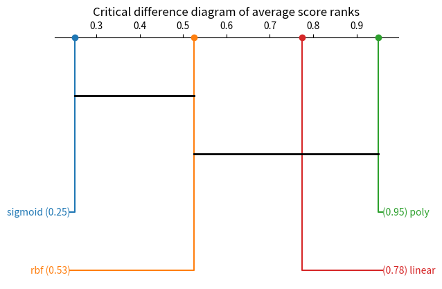
res = auto_kruskal_for_df(dfi, interesting_col=target, hue_col=treatment)
if res.pvalue < 0.05:
    print("There is a significant difference between the kernel functions.")
res

Sun 2024-12-01 22:26:57.502502

INFO     There is a significant difference between the kernel functions.                              nucleus.py:53

KruskalResult(statistic=89.11831011539, pvalue=3.3878339514086004e-19)

Kruskal-Wallis H-test tests的零假设是 不同组的中位数之间没有显著差异。看来我们可以拒绝原假设，认为不同kernel的SVM的中位数有显著差异。

刚才我们检验出来存在显著差异，但是不知道具体是谁比谁大有显著性，所以我们还需要使用post-hoc类型的假设检验来进行进一步的分析。

首先刚才检验的是中位数有显著差异，我们来求一下分组的中位数。

import pandas as pd

medians = df.groupby(treatment)[target].median().sort_values(ascending=False)
medians

params_kernel
poly           0.989559
linear         0.985383
sigmoid        0.650010
rbf            0.516373
precomputed         NaN
Name: value, dtype: float64

order = medians.index[:-1]

Dunn’s test就是针对 Kruskal-Wallis one-way analysis 对应的 post-hoc 检验方法（之一，还有其他的）。

import scikit_posthocs as sp
from scikit_posthocs import posthoc_dunn

res = posthoc_dunn(dfi, val_col=target, group_col=treatment, 
             sort=True, p_adjust='holm')

# 按照中位数大小排序
res = res.reindex(order)
res = res[order]
res

	poly	linear	sigmoid	rbf
params_kernel
poly	1.000000e+00	3.388027e-08	1.939419e-12	2.481610e-07
linear	3.388027e-08	1.000000e+00	6.615530e-02	1.597734e-01
sigmoid	1.939419e-12	6.615530e-02	1.000000e+00	9.446169e-01
rbf	2.481610e-07	1.597734e-01	9.446169e-01	1.000000e+00

# res < 0.05
heatmap_args = {'linewidths': 0.25, 'linecolor': '0.5', 'clip_on': False, 'square': True, 'cbar_ax_bbox': [0.80, 0.35, 0.04, 0.3]}
sp.sign_plot(res, **heatmap_args)

(<Axes: ylabel='params_kernel'>, <matplotlib.colorbar.Colorbar object at 0x7f3600724400>)

从结果表可以看出，poly非常显著地优于其他三个方法，是最好的方法。而linear虽然看起来中位数比剩下两个方法高，但是不显著。

以上的结果似乎不符合读者的直觉，你可能会说“kernel method不是很厉害吗，SVM重要的方法之一哎，怎么会不行呢？”

需要注意的是，我们刚才的实验随机采样了很多参数，kernel method也有厉害的参数，也有不厉害的参数。那我们刚才严格的假设检验如何解读呢？

正确的解读应该是这样的。假如有一个小白，不懂SVM，让他随机选择一个参数来调用sklearn库。我们是调过参的，我们告诉他，你是小白，如果你用rbf和sigmoid，你随便选别的参数，你很容易犯错误，让指标特别低。相反地，如果你用linear或者poly，你随便调其他的参数都无所谓，你大概率是能得到较好的结果的。

这就是我们上面的研究的意义，一个新的随机用户在随机场景下使用你的方法来替代其他方法时，他得到的期望改进。我们的结果就是 linear 和 poly的期望更高。但是这不意味着专家不能用rbf 和 sigmoid经过仔细调参得到更好的结果。

0.1.5.4 以 kernel 为目标元参数进行假设检验分析——最优对比分析

max_rows = dfi.loc[dfi.groupby(treatment)[target].idxmax()]
max_rows

	value	params_C	params_break_ties	params_class_weight	params_coef0	params_decision_function_shape	params_degree	params_gamma	params_kernel	params_max_iter	...	user_attrs_precision-run1	user_attrs_precision-run2	user_attrs_precision-run3	user_attrs_precision-run4	user_attrs_recall-mean	user_attrs_recall-run0	user_attrs_recall-run1	user_attrs_recall-run2	user_attrs_recall-run3	user_attrs_recall-run4
24	0.985383	60.429639	True	balanced	0.343750	ovr	6.0	scale	linear	656.0	...	0.990013	0.985716	0.974978	0.990491	0.984965	0.985093	0.988435	0.984900	0.975855	0.990541
5	0.990258	1.778279	False	None	0.250000	ovo	3.0	auto	poly	750.0	...	0.985863	0.988889	0.981481	1.000000	0.989942	0.991154	0.986591	0.989747	0.982219	1.000000
45	0.979820	77.736503	False	balanced	0.015625	ovo	4.0	auto	rbf	453.0	...	0.981515	0.985716	0.971346	0.983036	0.979199	0.972401	0.983471	0.984758	0.971617	0.983750
57	0.937369	0.835363	False	balanced	0.171875	ovr	2.0	scale	sigmoid	797.0	...	0.934272	0.942155	0.938151	0.939654	0.936771	0.942251	0.931733	0.938035	0.936699	0.935135

4 rows × 55 columns

critical_metric = "acc1_pred"
num_repeated = 5
kfold_metrics = [f"user_attrs_{critical_metric}-run{i}" for i in range(num_repeated)]

intereting_df =  max_rows[[treatment]+kfold_metrics]
intereting_df = intereting_df.set_index(treatment)
intereting_df

	user_attrs_acc1_pred-run0	user_attrs_acc1_pred-run1	user_attrs_acc1_pred-run2	user_attrs_acc1_pred-run3	user_attrs_acc1_pred-run4
params_kernel
linear	0.986111	0.989583	0.986063	0.975610	0.989547
poly	0.993056	0.986111	0.989547	0.982578	1.000000
rbf	0.975694	0.982639	0.986063	0.972125	0.982578
sigmoid	0.940972	0.934028	0.940767	0.937282	0.933798

analysis_df = intereting_df.transpose()
analysis_df = analysis_df.reset_index(drop=False)
analysis_df = analysis_df.rename(columns={analysis_df.columns[0]: 'runs'})
analysis_df = analysis_df.rename_axis('index')
analysis_df

params_kernel	runs	linear	poly	rbf	sigmoid
index
0	user_attrs_acc1_pred-run0	0.986111	0.993056	0.975694	0.940972
1	user_attrs_acc1_pred-run1	0.989583	0.986111	0.982639	0.934028
2	user_attrs_acc1_pred-run2	0.986063	0.989547	0.986063	0.940767
3	user_attrs_acc1_pred-run3	0.975610	0.982578	0.972125	0.937282
4	user_attrs_acc1_pred-run4	0.989547	1.000000	0.982578	0.933798

array_data = analysis_df.drop(analysis_df.columns[0], axis=1).values
array_data

array([[0.98611111, 0.99305556, 0.97569444, 0.94097222],
       [0.98958333, 0.98611111, 0.98263889, 0.93402778],
       [0.98606272, 0.98954704, 0.98606272, 0.94076655],
       [0.97560976, 0.9825784 , 0.97212544, 0.93728223],
       [0.98954704, 1.        , 0.9825784 , 0.93379791]])

analysis_df.columns[1]

'linear'

from scikit_posthocs import __convert_to_block_df

analysis_df_regular, _, _, _ = __convert_to_block_df(array_data)
analysis_df_regular = analysis_df_regular.rename(columns={'blocks': 'runs', 
                                                          'groups': treatment, 'y':target})
analysis_df_regular[treatment] = analysis_df_regular[treatment].apply(lambda x: analysis_df.columns[1+x])
analysis_df_regular

	runs	params_kernel	value
0	0	linear	0.986111
1	1	linear	0.989583
2	2	linear	0.986063
3	3	linear	0.975610
4	4	linear	0.989547
5	0	poly	0.993056
6	1	poly	0.986111
7	2	poly	0.989547
8	3	poly	0.982578
9	4	poly	1.000000
10	0	rbf	0.975694
11	1	rbf	0.982639
12	2	rbf	0.986063
13	3	rbf	0.972125
14	4	rbf	0.982578
15	0	sigmoid	0.940972
16	1	sigmoid	0.934028
17	2	sigmoid	0.940767
18	3	sigmoid	0.937282
19	4	sigmoid	0.933798

现在我们对五折交叉验证的结果来对四个方法进行假设检验。 这一次我们该使用 Friedman 检验, 这也是一个不需要正态性和方差齐性的检验方法，某种程度上论文会选择这个而非 Kruskal-Wallis。 刚才我们不用是因为刚才每一组的样本量不一致，而 Friedman 检验要求样本量一致

import scipy.stats as ss

res = ss.friedmanchisquare(*array_data.T)
if res.pvalue < 0.05:
    print("Reject null hypothesis. Therefore, the data is significantly different.")
res

Sun 2024-12-01 22:27:13.508583

INFO     Reject null hypothesis. Therefore, the data is significantly different.                      nucleus.py:53

FriedmanchisquareResult(statistic=13.653061224489791, pvalue=0.003417529443793913)

Nemenyi 是其中的一个 对应于 Friedman 的测试。

首先我们需要计算4个方法的平均排名（在同一个cv fold上，相互之间的排名），这个是 判断哪个方法更好的核心依据。

avg_rank = analysis_df_regular.groupby('runs').value.rank(pct=True).groupby(analysis_df_regular.params_kernel).mean().sort_values(ascending=False)
avg_rank

params_kernel
poly       0.950
linear     0.775
rbf        0.525
sigmoid    0.250
Name: value, dtype: float64

按照平均排名重新排序

analysis_df = analysis_df[avg_rank.index]
analysis_df

params_kernel	poly	linear	rbf	sigmoid
index
0	0.993056	0.986111	0.975694	0.940972
1	0.986111	0.989583	0.982639	0.934028
2	0.989547	0.986063	0.986063	0.940767
3	0.982578	0.975610	0.972125	0.937282
4	1.000000	0.989547	0.982578	0.933798

array_data = analysis_df.values
array_data

array([[0.99305556, 0.98611111, 0.97569444, 0.94097222],
       [0.98611111, 0.98958333, 0.98263889, 0.93402778],
       [0.98954704, 0.98606272, 0.98606272, 0.94076655],
       [0.9825784 , 0.97560976, 0.97212544, 0.93728223],
       [1.        , 0.98954704, 0.9825784 , 0.93379791]])

import scikit_posthocs as sp

# res = sp.posthoc_nemenyi_friedman(analysis_df_regular, 
#                                   block_col="runs", 
#                                   group_col=treatment, y_col=target, sort=True)
res = sp.posthoc_nemenyi_friedman(array_data) 
res

	0	1	2	3
0	1.000000	0.826788	0.158925	0.003389
1	0.826788	1.000000	0.611061	0.049612
2	0.158925	0.611061	1.000000	0.532733
3	0.003389	0.049612	0.532733	1.000000

sp.sign_plot(res, xticklabels=avg_rank.index, yticklabels=avg_rank.index, **heatmap_args)

(<Axes: >, <matplotlib.colorbar.Colorbar object at 0x7f3620291390>)

从检验的结果图可以看出，poly和linear方法明显优于sigmoid，而其他方法之间就没有足够的实验证据来进行比较。 这说明sigmoid方法即使调到了较优的超参数，还是显著比前两个方法要弱一些，不建议新手使用。

plt.title('Critical difference diagram of average score ranks')
sp.critical_difference_diagram(avg_rank, res)
pass

我们还画出了 Critical difference diagram。 图中靠右边的方法平均排名高，左边的方法平均排名低。 排名的差距是否具有统计上的显著性，关键看差距是否大于图中的黑色实线的长度。

我们可以看到poly几乎就要显著优于rbf了，而rbf几乎就要显著优于sigmoid了，但是都还差一点不太显著。

0.1.5.5 如何解释 poly kernel 为什么显著优于 sigmoid kernel? SVM决策边界可视化分析

如果是2维或者3维的数据，我们可以画图来解释SVM工作的原理，绘制决策边界，但是我们现在是 64维 (UCI digits) 或者 728维 (MNIST) 的输入数据。这一方面可以参考这一个工具mlxtend，对SVM的可视化非常全面。

对于深度学习模型来说，深度学习最后一层的特征往往被认为是表示学习的结果，用来进行降维可视化，但是我们这里 SVM 是单层的模型，没有对特征进行变换，输入的维度就已经是特征。直接对输入的数据特征进行降维可视化，完全无法展示SVM的能力，因为SVM并不是一个特征提取器。

综合stackoverflow讨论 和 quora讨论，我认为有两个主要方法。

• 对降维后的数据重新使用不同kernel的SVM来学习，进一步绘制决策边界。使用刚才每一个kernel下调参最优的SVM参数来进行训练。
• SVM的概率输出，概率本身就是一个重要的信息，体现了不同SVM的决策有何不同。类似与Fisher提出的LDA分类方法自己也是一种降维方法，带概率输出的SVM把输入维度映射到类别维度上的概率值，本身是一种降维手法，而且体现了不同参数SVM的学习有何不同。

如果不是为了看SVM的能力，而是为了解释kernel method的能力，我们还可以使用 KernelPCA 的可视化进行分析。

首先我们调取最优的训练参数

from sklearn.svm import SVC

# 提取以 'params_' 开头的列
param_cols = [col for col in max_rows.columns if col.startswith('params_')]

# 去掉 'params_' 前缀并重命名列
max_rows_params = max_rows[param_cols].rename(columns=lambda x: x[len('params_'):])

# 将每一行转换为字典的列表
dict_list = max_rows_params.to_dict('records')
dict_list[0]

{
    'C': 60.42963902381333,
    'break_ties': True,
    'class_weight': 'balanced',
    'coef0': 0.34375,
    'decision_function_shape': 'ovr',
    'degree': 6.0,
    'gamma': 'scale',
    'kernel': 'linear',
    'max_iter': 656.0,
    'shrinking': True,
    'tol': 0.008058421877614822
}

optuna优化时，把数据类型有些变成了float，需要更正。

from dataclasses import fields
from typing import get_args, Union

---

source

dict_to_dataclass

 dict_to_dataclass (dataclass_type, data_dict)

def dict_to_dataclass(dataclass_type, data_dict):
    converted_dict = {}
    for field in fields(dataclass_type):
        field_name = field.name
        field_type = field.type
        if field_name in data_dict:
            value = data_dict[field_name]
            # 处理 Union 类型
            if getattr(field_type, '__origin__', None) is Union:
                # 获取 Union 中的所有类型
                types = get_args(field_type)
                # 选择第一个非 NoneType 的类型
                non_none_types = [t for t in types if t is not type(None)]
                target_type = non_none_types[0] if non_none_types else None
                # print(target_type)
                if target_type not in [dict, list, tuple]: # TODO 递归处理
                    converted_dict[field_name] = target_type(value)
                else:
                    converted_dict[field_name] = value
            else:
                converted_dict[field_name] = field_type(value)
    return dataclass_type(**converted_dict)

# 将 dict_list 中的参数转换为 SupportVectorClassifierConfig 的实例列表
configs = [dict_to_dataclass(SupportVectorClassifierConfig, params) for params in dict_list]
# 根据 dict_list 初始化 SVC 列表
svc_list = [SVC(**asdict(config)) for config in configs]
svc_list[0]

SVC(C=60.42963902381333, break_ties=True, class_weight='balanced',
    coef0=0.34375, degree=6, kernel='linear', max_iter=656,
    tol=0.008058421877614822)

In a Jupyter environment, please rerun this cell to show the HTML representation or trust the notebook.
On GitHub, the HTML representation is unable to render, please try loading this page with nbviewer.org.

然后我们先使用第一种分析方法，做降维。

from sklearn.decomposition import PCA

# 定义 PCA 模型，设定降维后的维度，例如 n_components=10
pca = PCA(n_components=2)

# 对 X_train 进行降维
X_train_reduced = pca.fit_transform(X_train)

# 对 X_test 进行降维
X_test_reduced = pca.transform(X_test)

# 查看 pca 的一些指标
pca.explained_variance_ratio_

array([0.12330114, 0.10126638], dtype=float32)

可视化

labels = [svc.kernel for svc in svc_list]
labels[0]

'linear'

import matplotlib.pyplot as plt
from mlxtend.plotting import plot_decision_regions
import matplotlib.gridspec as gridspec
import itertools

gs = gridspec.GridSpec(2, 2)

fig = plt.figure(figsize=(10,8))

for clf, lab, grd in zip(svc_list,
                         labels,
                         itertools.product([0, 1], repeat=2)):

    clf.fit(X_train_reduced, y_train)
    ax = plt.subplot(gs[grd[0], grd[1]])
    fig = plot_decision_regions(X=X_train_reduced, y=y_train, clf=clf, legend=2)
    plt.title(lab)

plt.show()

0.1.5.6 如何解释 poly kernel 为什么显著优于 sigmoid kernel? Kernel SVM概率输出的画图分析

首先在没有降维的数据集上按照最优参数来训练SVC。注意为了速度，刚才调参的时候没有probality=True，现在为了分析需要有。

svc_list = [SVC(**(asdict(config)| dict(probability=True)) )  for config in configs]
svc_list = [svc.fit(X_train, y_train) for svc in svc_list]

得到 y_pred_prob

y_pred_train_probs = [svc.predict_proba(X_train) for svc in svc_list]
y_pred_test_probs = [svc.predict_proba(X_test) for svc in svc_list]

---

source

draw_probs

 draw_probs (y_pred_prob, y_test, interested_class:int)

import seaborn as sns

def draw_probs(y_pred_prob, y_test, interested_class:int):
    sns.scatterplot(y_pred_prob[y_test!=interested_class][:, interested_class], label=f"is not {interested_class}")
    sns.scatterplot(y_pred_prob[y_test==interested_class][:, interested_class], label=f"is {interested_class}", color="red")

# 对所有的 y_pred_train_probs 和 y_pred_test_probs，调用 draw_probs 函数并绘制图形
# intersted_class = 0
intersted_class = 3
for i, model_name in enumerate(labels):
    train_probs = y_pred_train_probs[i]
    test_probs = y_pred_test_probs[i]
    
    # 创建左右并排的图形
    plt.figure(figsize=(12, 5))
    
    # 绘制训练集的概率分布图
    plt.subplot(1, 2, 1)
    draw_probs(train_probs, y_train, interested_class=intersted_class)
    plt.title(f'{model_name} - Training Set')
    
    # 绘制测试集的概率分布图
    plt.subplot(1, 2, 2)
    draw_probs(test_probs, y_test, interested_class=intersted_class)
    plt.title(f'{model_name} - Test Set')
    
    plt.tight_layout()
    plt.show()

我们在图上可以比较明显地看出，sigmoid相比其他方法，probabilities 会往上和往下飘，是否为这个类别的分隔的不是很开，所以最后的效果不如poly。而其他方法可能测试集会稍微没有训练集分隔得开。

除了直接画出来概率的散点图，还有一些更加成熟的机器学习绘图分析，可以更加直观地看到模型的差距在哪。

import scikitplot as skplt
import scikitplot as skplt
import matplotlib.pyplot as plt

# 假设 labels 是模型名称的列表，与预测概率列表对应
# labels = ['linear', 'poly', 'rbf', 'sigmoid']

for i, model_name in enumerate(labels):
    train_probs = y_pred_train_probs[i]
    test_probs = y_pred_test_probs[i]
    
    # 创建左右并排的图形
    fig, (ax1, ax2) = plt.subplots(1, 2, figsize=(12, 5))
    
    # 绘制训练集的 ROC 曲线
    skplt.metrics.plot_roc(y_train, train_probs, ax=ax1)
    ax1.set_title(f'{model_name} - Training Set')
    
    # 绘制测试集的 ROC 曲线
    skplt.metrics.plot_roc(y_test, test_probs, ax=ax2)
    ax2.set_title(f'{model_name} - Test Set')
    
    plt.tight_layout()
    plt.show()

图中可以明显看到 sigmoid kernel方法在 类别 1和8上面表现不佳。而poly的曲线接近完美。

0.1.5.7 如何解释 poly kernel 为什么显著优于 sigmoid kernel? Kernel PCA 可视化

from sklearn.decomposition import KernelPCA
import matplotlib.pyplot as plt
from mpl_toolkits.mplot3d import Axes3D

# labels = ['linear', 'poly', 'rbf', 'sigmoid']

for kernel in labels:
    # 使用 Kernel PCA 将数据降维到 3 维
    kpca = KernelPCA(n_components=3, kernel=kernel)
    X_train_reduced = kpca.fit_transform(X_train)
    X_test_reduced = kpca.transform(X_test)
    
    # 创建一个包含两个子图的图形
    fig = plt.figure(figsize=(12, 6))
    
    # 绘制训练集的 3D 散点图
    ax1 = fig.add_subplot(1, 2, 1, projection='3d')
    scatter1 = ax1.scatter(
        X_train_reduced[:, 0], X_train_reduced[:, 1], X_train_reduced[:, 2],
        c=y_train, cmap='viridis', marker='o', edgecolor='k', s=40
    )
    ax1.set_title(f'Kernel PCA with {kernel} kernel (Training Set)')
    ax1.set_xlabel('Component 1')
    ax1.set_ylabel('Component 2')
    ax1.set_zlabel('Component 3')
    legend1 = ax1.legend(*scatter1.legend_elements(), title="Classes")
    ax1.add_artist(legend1)
    
    # 绘制测试集的 3D 散点图
    ax2 = fig.add_subplot(1, 2, 2, projection='3d')
    scatter2 = ax2.scatter(
        X_test_reduced[:, 0], X_test_reduced[:, 1], X_test_reduced[:, 2],
        c=y_test, cmap='viridis', marker='^', edgecolor='k', s=40
    )
    ax2.set_title(f'Kernel PCA with {kernel} kernel (Test Set)')
    ax2.set_xlabel('Component 1')
    ax2.set_ylabel('Component 2')
    ax2.set_zlabel('Component 3')
    legend2 = ax2.legend(*scatter2.legend_elements(), title="Classes")
    ax2.add_artist(legend2)
    
    plt.tight_layout()
    plt.show()

0.2 附加题: 构建使用 kernel 方法的 SVM 分类器 （手动实现SMO）

在 02svm_handy_crafted_linear 中，我们已经手动实现了 基于梯度下降方法的 Linear SVM 分类器。在这一节，我们将手动实现 基于 SMO 方法的 SVM 分类器，以便于我们可以更好地理解 SVM 的原理。

接下来的内容请见文件 04svm_handy_crafted_kernel

本次Project的目录请见绪论 00svm。